  General_Health                 Checkup Exercise Heart_Disease Skin_Cancer
1           Poor Within the past 2 years       No            No          No
2      Very Good    Within the past year       No           Yes          No
3      Very Good    Within the past year      Yes            No          No
4           Poor    Within the past year      Yes           Yes          No
5           Good    Within the past year       No            No          No
6           Good    Within the past year       No            No          No
  Other_Cancer Depression Diabetes Arthritis    Sex Age_Category Height_.cm.
1           No         No       No       Yes Female        70-74         150
2           No         No      Yes        No Female        70-74         165
3           No         No      Yes        No Female        60-64         163
4           No         No      Yes        No   Male        75-79         180
5           No         No       No        No   Male          80+         191
6           No        Yes       No       Yes   Male        60-64         183
  Weight_.kg.   BMI Smoking_History Alcohol_Consumption Fruit_Consumption
1       32.66 14.54             Yes                   0                30
2       77.11 28.29              No                   0                30
3       88.45 33.47              No                   4                12
4       93.44 28.73              No                   0                30
5       88.45 24.37             Yes                   0                 8
6      154.22 46.11              No                   0                12
  Green_Vegetables_Consumption FriedPotato_Consumption
1                           16                      12
2                            0                       4
3                            3                      16
4                           30                       8
5                            4                       0
6                           12                      12
Selecting a subset of participants from CVD: 20000 participants
Number_ofparticipants <-10000## This is a very large dataset, let's only select 10000 samples from both groupsset.seed(150)Yes_case <-sample(which(Heart_data$Heart_Disease =="Yes"), Number_ofparticipants)set.seed(150)No_case <-sample(which(Heart_data$Heart_Disease =="No"), Number_ofparticipants)Data_yes <- Heart_data[Yes_case, ]Data_no <- Heart_data[No_case, ]Data_total <-rbind(Data_yes, Data_no)head(Data_total)
       General_Health              Checkup Exercise Heart_Disease Skin_Cancer
43289            Poor Within the past year      Yes           Yes         Yes
281436           Fair Within the past year      Yes           Yes          No
196610           Fair Within the past year      Yes           Yes          No
306903           Fair Within the past year       No           Yes          No
304887           Poor Within the past year       No           Yes          No
278988           Fair Within the past year      Yes           Yes          No
       Other_Cancer Depression Diabetes Arthritis    Sex Age_Category
43289            No         No      Yes       Yes   Male        65-69
281436           No         No      Yes       Yes   Male        70-74
196610           No         No      Yes       Yes Female        40-44
306903          Yes         No      Yes       Yes Female        55-59
304887           No        Yes       No       Yes   Male          80+
278988           No         No       No        No   Male        50-54
       Height_.cm. Weight_.kg.   BMI Smoking_History Alcohol_Consumption
43289          175      102.97 33.52             Yes                   0
281436         170      104.33 36.02             Yes                   0
196610         180      136.08 41.84             Yes                   5
306903         160       65.77 25.69              No                   0
304887         155       62.60 26.07             Yes                   0
278988         180      106.59 32.78              No                  25
       Fruit_Consumption Green_Vegetables_Consumption FriedPotato_Consumption
43289                 12                           16                       3
281436                60                           30                       4
196610                60                            2                      12
306903                12                           12                       3
304887                28                           28                       4
278988                 3                            4                       8
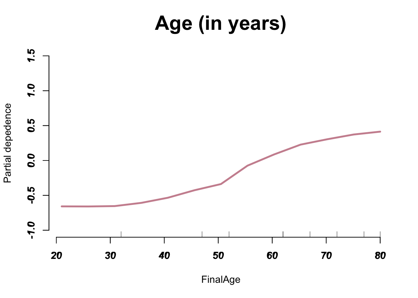
Converting Age from range to numerical value
## We will convert the Age variable that is in range form in the dataset to a numerical form.My_Age_Heart_Data <-data.frame(Data_total$Age_Category, Data_total$Heart_Disease)names(My_Age_Heart_Data) <-c("Age_Category", "Heart_Disease") # This code gets the data in the right formatMy_Age_Heart_Data$Age_min <-as.numeric(substr(My_Age_Heart_Data$Age_Category, start =1, stop =2))My_Age_Heart_Data$Age_max <-as.numeric(substr(My_Age_Heart_Data$Age_Category, start =4, stop =5))for (i in1:Number_ofparticipants){# if (is.na(My_Age_Heart_Data$Age_min[i])){# My_Age_Heart_Data$Age_min[i] = My_Age_Heart_Data$Age_max[i]}if (is.na(My_Age_Heart_Data$Age_max[i])){ My_Age_Heart_Data$Age_max[i] = My_Age_Heart_Data$Age_min[i]}}## We check if there were other missing age value included in the data.more_missing_agevalue <- Data_total$Age_Category[(is.na(My_Age_Heart_Data$Age_max))]## Since all the missing values were participants 80 and older, we replace those missing values with 80.My_Age_Heart_Data$Age_max[(is.na(My_Age_Heart_Data$Age_max))] =as.numeric(80)# This code gives me the final age value to be used in the analysis.My_Age_Heart_Data$FinalAge <- (My_Age_Heart_Data$Age_min + My_Age_Heart_Data$Age_max)/2head(My_Age_Heart_Data)
## Here we will remove the Diabetes column that do not make sense to us. Extra_DiabetesandnullAge_Column <-which((Data_total$Diabetes =="Yes, but female told only during pregnancy") | (Data_total$Diabetes =="No, pre-diabetes or borderline diabetes"))## This is our final data with clean variablesData_total <- Data_total[-Extra_DiabetesandnullAge_Column, ]Data_total$Diabetes <-factor(Data_total$Diabetes)Data_total$Age_Category <-NULL# removing age categorystr(Data_total)
Call:
randomForest(formula = HeartLabel_Train ~ ., data = train_data, ntree = 500, proximity = T, mtry = 3)
Type of random forest: classification
Number of trees: 500
No. of variables tried at each split: 3
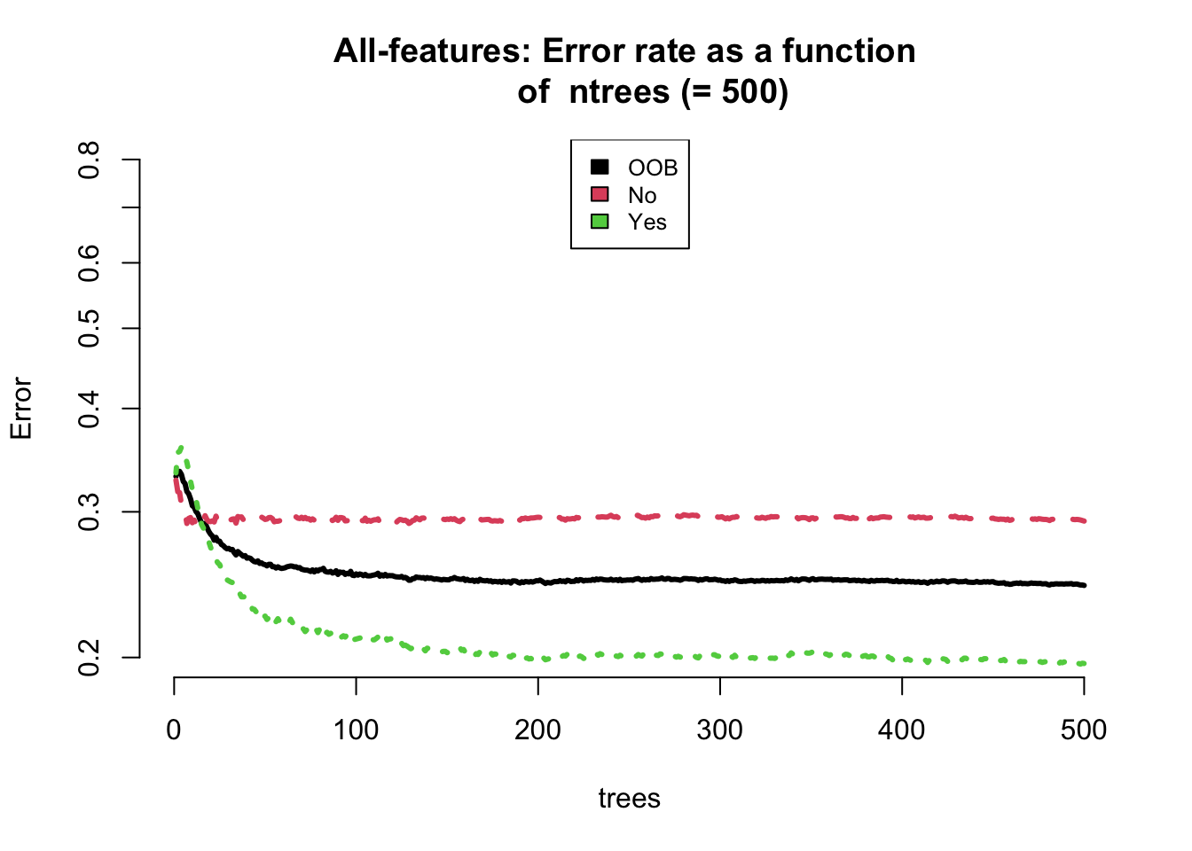
OOB estimate of error rate: 24.44%
Confusion matrix:
No Yes class.error
No 4775 1973 0.2923829
Yes 1333 5445 0.1966657
Parameter Tuning
## Parameter Tuning A: here we find the optimal number of decision treesplot(our_model_500, log ="y", main ="All-features: Error rate as a function of ntrees (= 500)", lwd =3, bty ="n", ylim =c(0.2,0.8))legend("top", colnames(our_model_500$err.rate), col =1:3, cex =0.8, fill =1:3)
## This is our random forest model with all featuresour_model_1000 <-randomForest(HeartLabel_Train ~ ., data = train_data, ntree =1000, proximity = T, mtry =3)our_model_1000
Call:
randomForest(formula = HeartLabel_Train ~ ., data = train_data, ntree = 1000, proximity = T, mtry = 3)
Type of random forest: classification
Number of trees: 1000
No. of variables tried at each split: 3
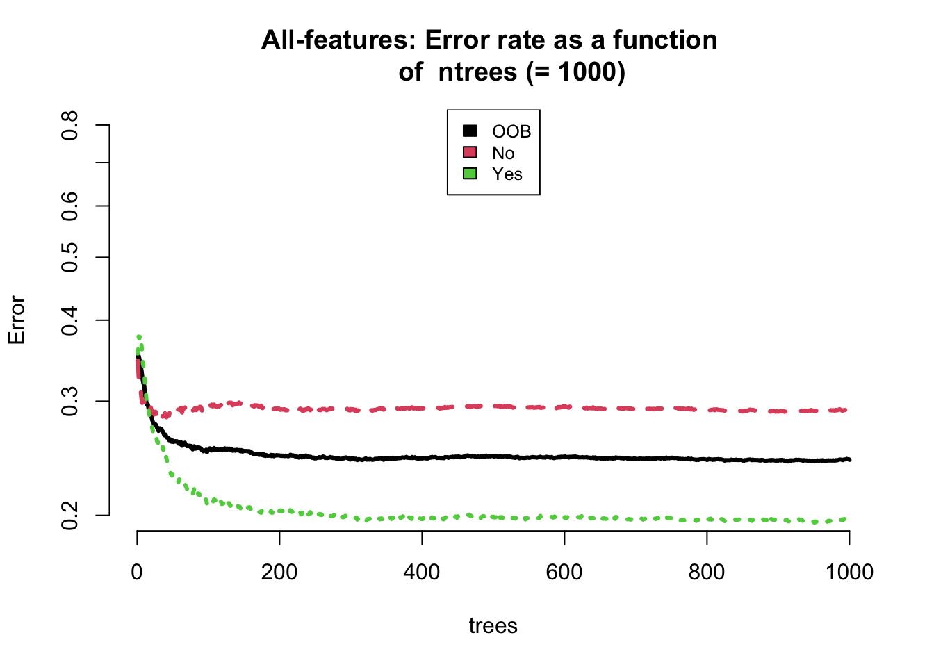
OOB estimate of error rate: 24.35%
Confusion matrix:
No Yes class.error
No 4786 1962 0.2907528
Yes 1332 5446 0.1965181
plot(our_model_1000, log ="y", main ="All-features: Error rate as a function of ntrees (= 1000)", lwd =3, bty ="n", ylim =c(0.2,0.8))legend("top", colnames(our_model_1000$err.rate), col =1:3, cex =0.8, fill =1:3)
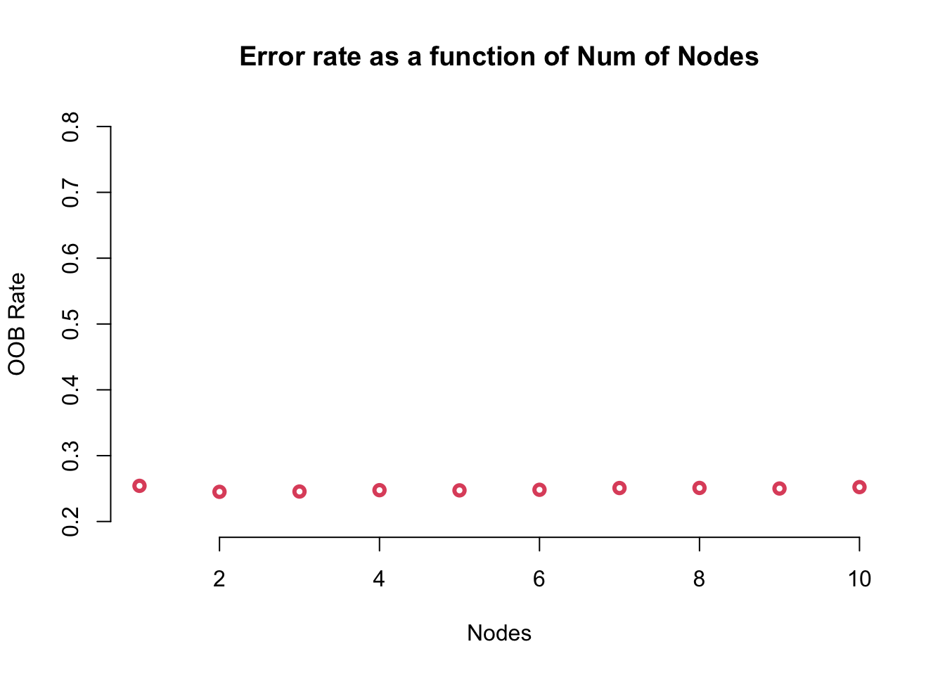
## Parameter Tuning B: now we will find the optimal number of split of the treeoob_values <-vector(length =10)for (i in1:10) { Num_model <-randomForest(HeartLabel_Train ~ ., data = train_data, mtry = i, ntree =500) oob_values[i] <- Num_model$err.rate[nrow(Num_model$err.rate), 1]}plot(oob_values, main ="Error rate as a function of Num of Nodes", lwd =3, bty ="n",ylim =c(0.2,0.8), col =2, xlab ="Nodes", ylab ="OOB Rate")
We will record the out of bag error estimate of the optimal model
Call:
 randomForest(formula = HeartLabel_Train ~ ., data = train_data,      ntree = 500, proximity = T, mtry = 2)
               Type of random forest: classification
                     Number of trees: 500
No. of variables tried at each split: 2

        OOB estimate of  error rate: 24.43%
Confusion matrix:
      No  Yes class.error
No  4726 2022   0.2996443
Yes 1282 5496   0.1891413
Model Features and Performance
Model Performance on the testing and training set
## Testing the model accuracy on the training datatrain_rf <-predict(our_model_500, train_data)Train_Summary <-confusionMatrix(train_rf, HeartLabel_Train)Train_Summary
Confusion Matrix and Statistics

          Reference
Prediction   No  Yes
       No  6091  384
       Yes  657 6394

               Accuracy : 0.923
                 95% CI : (0.9184, 0.9275)
    No Information Rate : 0.5011
    P-Value [Acc > NIR] : < 2.2e-16

                  Kappa : 0.8461

 Mcnemar's Test P-Value : < 2.2e-16

            Sensitivity : 0.9026
            Specificity : 0.9433
         Pos Pred Value : 0.9407
         Neg Pred Value : 0.9068
             Prevalence : 0.4989
         Detection Rate : 0.4503
   Detection Prevalence : 0.4787
      Balanced Accuracy : 0.9230

       'Positive' Class : No
## Testing the model accuracy on the testing datatest_rf <-predict(our_model_500, test_data)Test_Summary <-confusionMatrix(test_rf, HeartLabel_Test)Test_Summary ## All features
Confusion Matrix and Statistics

          Reference
Prediction   No  Yes
       No  2022  541
       Yes  904 2330

               Accuracy : 0.7507
                 95% CI : (0.7394, 0.7618)
    No Information Rate : 0.5047
    P-Value [Acc > NIR] : < 2.2e-16

                  Kappa : 0.502

 Mcnemar's Test P-Value : < 2.2e-16

            Sensitivity : 0.6910
            Specificity : 0.8116
         Pos Pred Value : 0.7889
         Neg Pred Value : 0.7205
             Prevalence : 0.5047
         Detection Rate : 0.3488
   Detection Prevalence : 0.4421
      Balanced Accuracy : 0.7513

       'Positive' Class : No
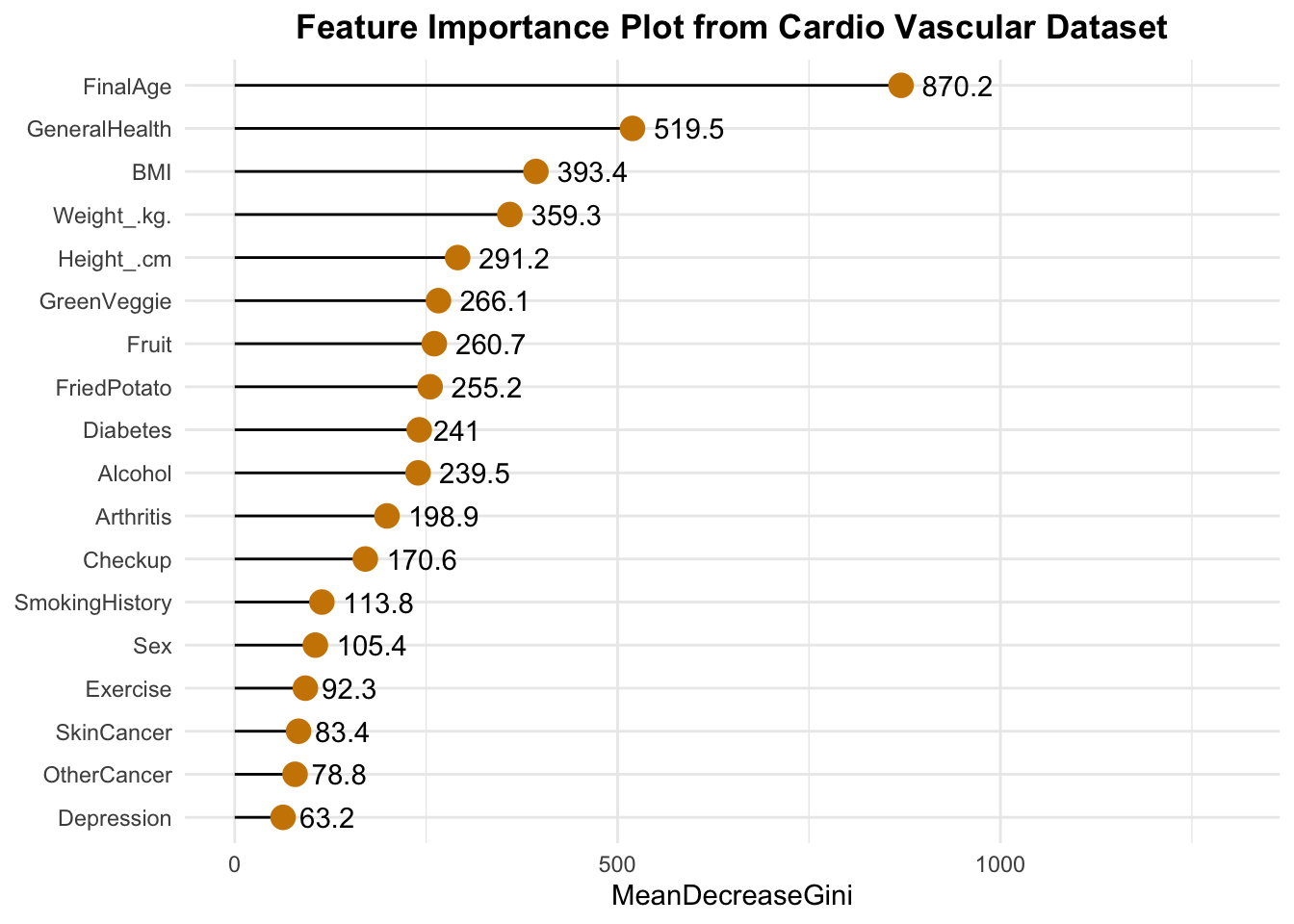
Which variables are most important according to our model
#install.packages("ggalt")suppressPackageStartupMessages({library(ggalt)library(randomForest)library(data.table)})## Here we get a nice looking plot for the feature important indeximp <-data.table(importance(our_model_500), keep.rownames =TRUE)imp =arrange(imp, MeanDecreaseGini)imp[, rn :=factor(rn, unique(rn))]ggplot(melt(imp, id.vars="rn")[grep("Mean", variable)], aes(x=rn, y=value, label =round(value, 1))) +geom_lollipop(point.size =4, point.colour ="orange3", pch =19, bg =2) +geom_text(aes(nudge_y =2), hjust =-.3) +coord_flip() +#facet_wrap(~variable) +theme_minimal() +labs(y="MeanDecreaseGini", x=NULL, title ="Feature Importance Plot from Cardio Vascular Dataset", cex =0.9) +expand_limits(y =1300) +theme(plot.title =element_text(face ="bold", hjust =0.5))