library(haven)
TEDS_2016 <-
read_stata("https://github.com/datageneration/home/blob/master/DataProgramming/data/TEDS_2016.dta?raw=true")Assignment3
Loading necessary packages and the data
Dealing with missing values
Checking missing values and removing rows with any missing data
sum(is.na(TEDS_2016))[1] 3008TEDS_2016_complete <- TEDS_2016[complete.cases(TEDS_2016), ]checking if data is in string and converting them to numeric if necessary
sum(is.na(TEDS_2016_complete))[1] 0TEDS_2016_complete <- TEDS_2016[complete.cases(TEDS_2016), ]
str(TEDS_2016_complete$age) num [1:1074] 39 63 64 75 54 64 66 41 57 43 ...
- attr(*, "format.stata")= chr "%9.0g"str(TEDS_2016_complete$income) num [1:1074] 7 8 9 1 10 2 3 9 1 5 ...
- attr(*, "format.stata")= chr "%9.0g"str(TEDS_2016_complete$edu) num [1:1074] 5 5 2 1 5 1 1 5 5 5 ...
- attr(*, "format.stata")= chr "%9.0g"TEDS_2016_complete$age <- as.numeric(TEDS_2016_complete$age)
TEDS_2016_complete$income <- as.numeric(TEDS_2016_complete$income)
TEDS_2016_complete$edu <- as.numeric(TEDS_2016_complete$edu)Running linear model on the data
attach(TEDS_2016_complete)
First_model <- lm(Edu ~ Age + income, data = TEDS_2016_complete)
summary(First_model)
Call:
lm(formula = Edu ~ Age + income, data = TEDS_2016_complete)

Residuals:
     Min       1Q   Median       3Q      Max
-2.96323 -0.86202  0.01732  0.75658  3.13798

Coefficients:
            Estimate Std. Error t value Pr(>|t|)
(Intercept)  4.52360    0.11461   39.47   <2e-16 ***
Age         -0.56033    0.02448  -22.89   <2e-16 ***
income       0.14007    0.01126   12.44   <2e-16 ***
---
Signif. codes:  0 '***' 0.001 '**' 0.01 '*' 0.05 '.' 0.1 ' ' 1

Residual standard error: 1.097 on 1071 degrees of freedom
Multiple R-squared:  0.4365,    Adjusted R-squared:  0.4354
F-statistic: 414.8 on 2 and 1071 DF, p-value: < 2.2e-16plot(Age, Edu)
abline(First_model, col = "red3")Warning in abline(First_model, col = "red3"): only using the first two of 3
regression coefficients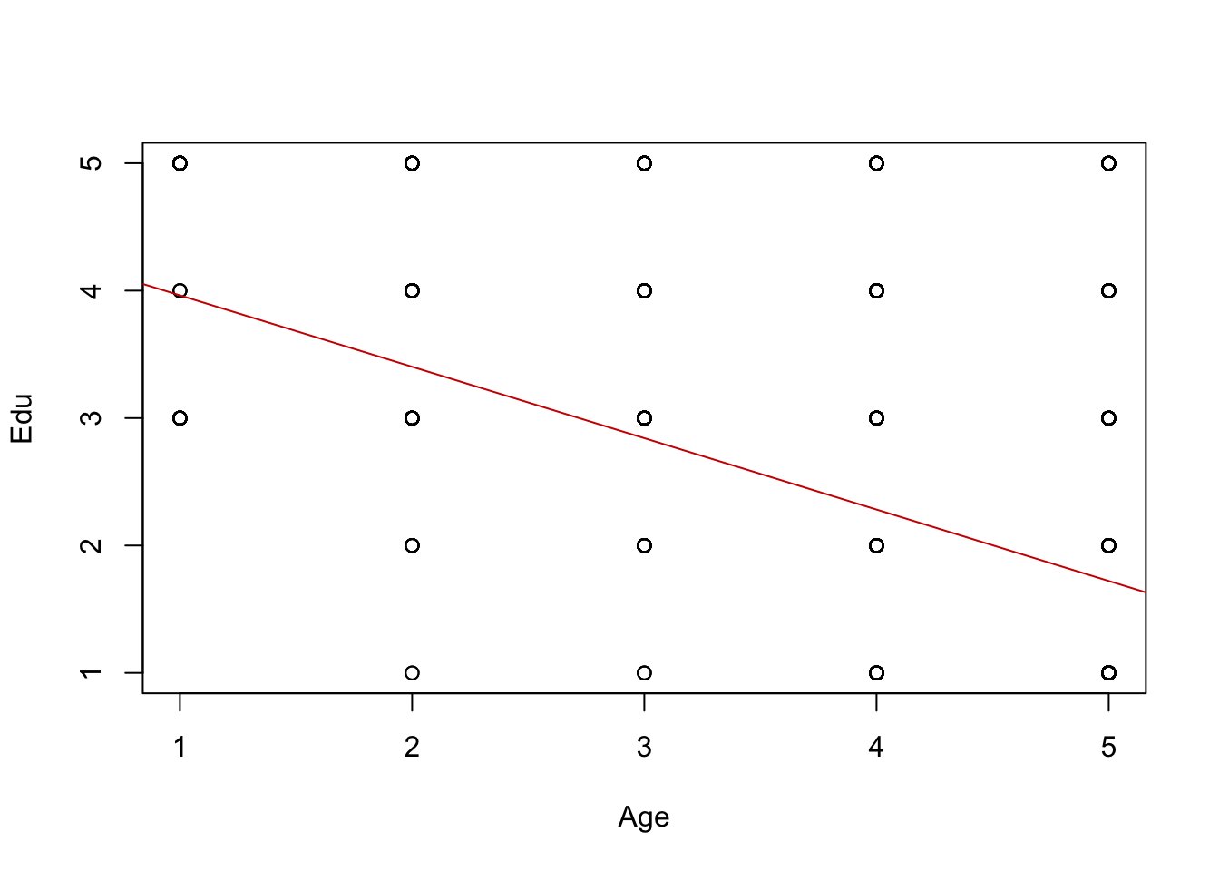
Second_model <- lm(Edu ~ income, data = TEDS_2016_complete)
summary(Second_model)
Call:
lm(formula = Edu ~ income, data = TEDS_2016_complete)

Residuals:
    Min      1Q  Median      3Q     Max
-3.3311 -0.9821  0.2106  1.0543  2.4034

Coefficients:
            Estimate Std. Error t value Pr(>|t|)
(Intercept)  2.40391    0.08237   29.18   <2e-16 ***
income       0.19272    0.01345   14.33   <2e-16 ***
---
Signif. codes:  0 '***' 0.001 '**' 0.01 '*' 0.05 '.' 0.1 ' ' 1

Residual standard error: 1.338 on 1072 degrees of freedom
Multiple R-squared:  0.1608,    Adjusted R-squared:   0.16
F-statistic: 205.4 on 1 and 1072 DF, p-value: < 2.2e-16plot(Age, Edu)
abline(First_model, col = "orange3")Warning in abline(First_model, col = "orange3"): only using the first two of 3
regression coefficients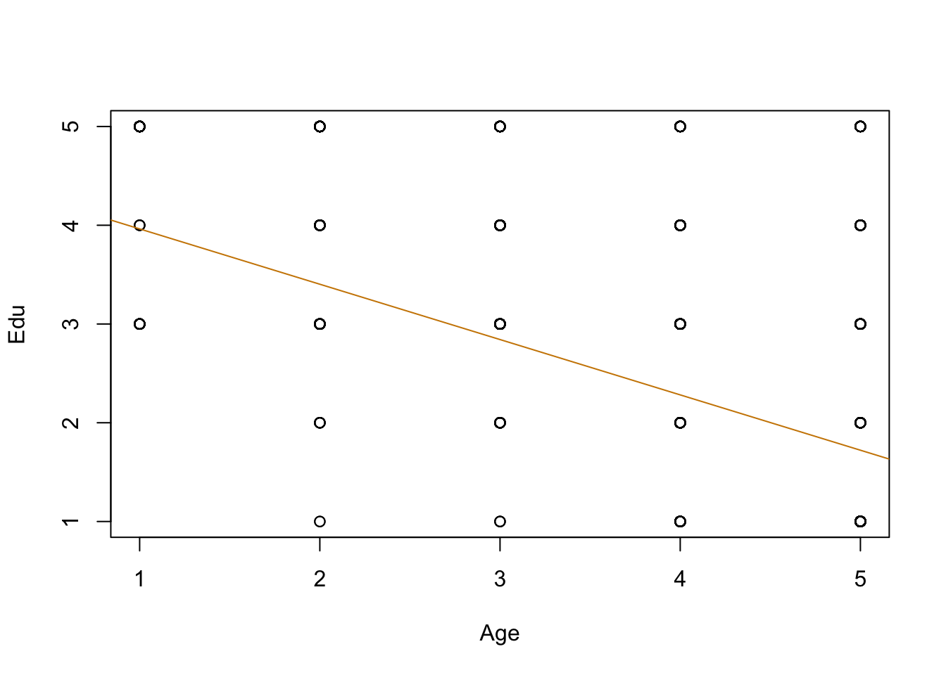
We removed the missing values and used the lm function to see how two predictors influence the outcome.
Tondu variable, then frequency and barchart on Tondu
TEDS_2016$Tondu<- as.numeric(TEDS_2016$Tondu,labels=c("Unification now”,
“Status quo, unif. in future”, “Status quo, decide later", "Status quo
forever", "Status quo, indep. in future", "Independence now”, “No response"))