# Prediction interval uses sample mean and takes into account the variability of the estimators for μ and σ.# Therefore, the interval will be wider.### Multiple linear regressionfit2=lm(medv~lstat+age,data=Boston)summary(fit2)
Call:
lm(formula = medv ~ lstat + age, data = Boston)

Residuals:
    Min      1Q  Median      3Q     Max
-15.981  -3.978  -1.283   1.968  23.158

Coefficients:
            Estimate Std. Error t value Pr(>|t|)
(Intercept) 33.22276    0.73085  45.458  < 2e-16 ***
lstat       -1.03207    0.04819 -21.416  < 2e-16 ***
age          0.03454    0.01223   2.826  0.00491 **
---
Signif. codes:  0 '***' 0.001 '**' 0.01 '*' 0.05 '.' 0.1 ' ' 1

Residual standard error: 6.173 on 503 degrees of freedom
Multiple R-squared:  0.5513,    Adjusted R-squared:  0.5495
F-statistic:   309 on 2 and 503 DF,  p-value: < 2.2e-16
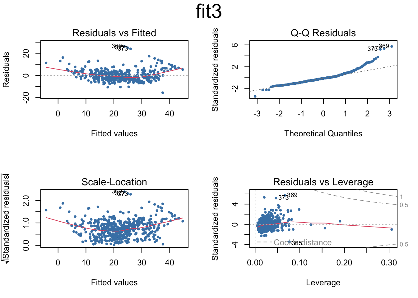
# Set the next plot configurationpar(mfrow=c(2,2), main="fit4")
Warning in par(mfrow = c(2, 2), main = "fit4"): "main" is not a graphical
parameter
plot(fit4,pch=20, cex=.8, col="steelblue")mtext("fit4", side =3, line =-2, cex =2, outer =TRUE)
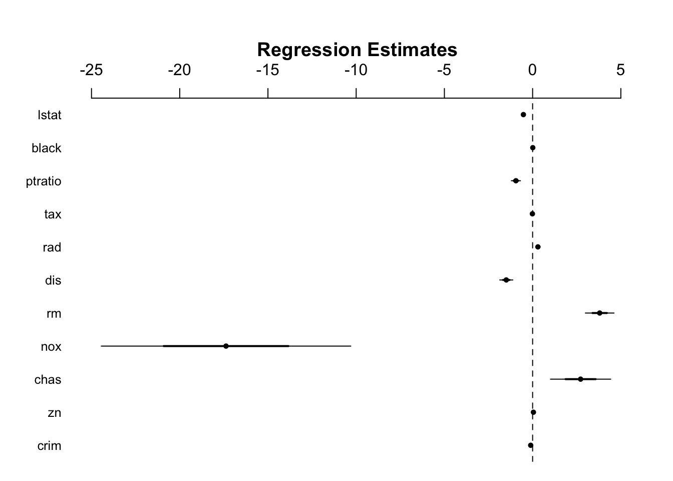
# Uses coefplot to plot coefficients. Note the line at 0.par(mfrow=c(1,1))arm::coefplot(fit4)
### Nonlinear terms and Interactionsfit5=lm(medv~lstat*age,Boston) # include both variables and the interaction term x1:x2summary(fit5)
Call:
lm(formula = medv ~ lstat * age, data = Boston)

Residuals:
    Min      1Q  Median      3Q     Max
-15.806  -4.045  -1.333   2.085  27.552

Coefficients:
              Estimate Std. Error t value Pr(>|t|)
(Intercept) 36.0885359  1.4698355  24.553  < 2e-16 ***
lstat       -1.3921168  0.1674555  -8.313 8.78e-16 ***
age         -0.0007209  0.0198792  -0.036   0.9711
lstat:age    0.0041560  0.0018518   2.244   0.0252 *
---
Signif. codes:  0 '***' 0.001 '**' 0.01 '*' 0.05 '.' 0.1 ' ' 1

Residual standard error: 6.149 on 502 degrees of freedom
Multiple R-squared:  0.5557,    Adjusted R-squared:  0.5531
F-statistic: 209.3 on 3 and 502 DF,  p-value: < 2.2e-16
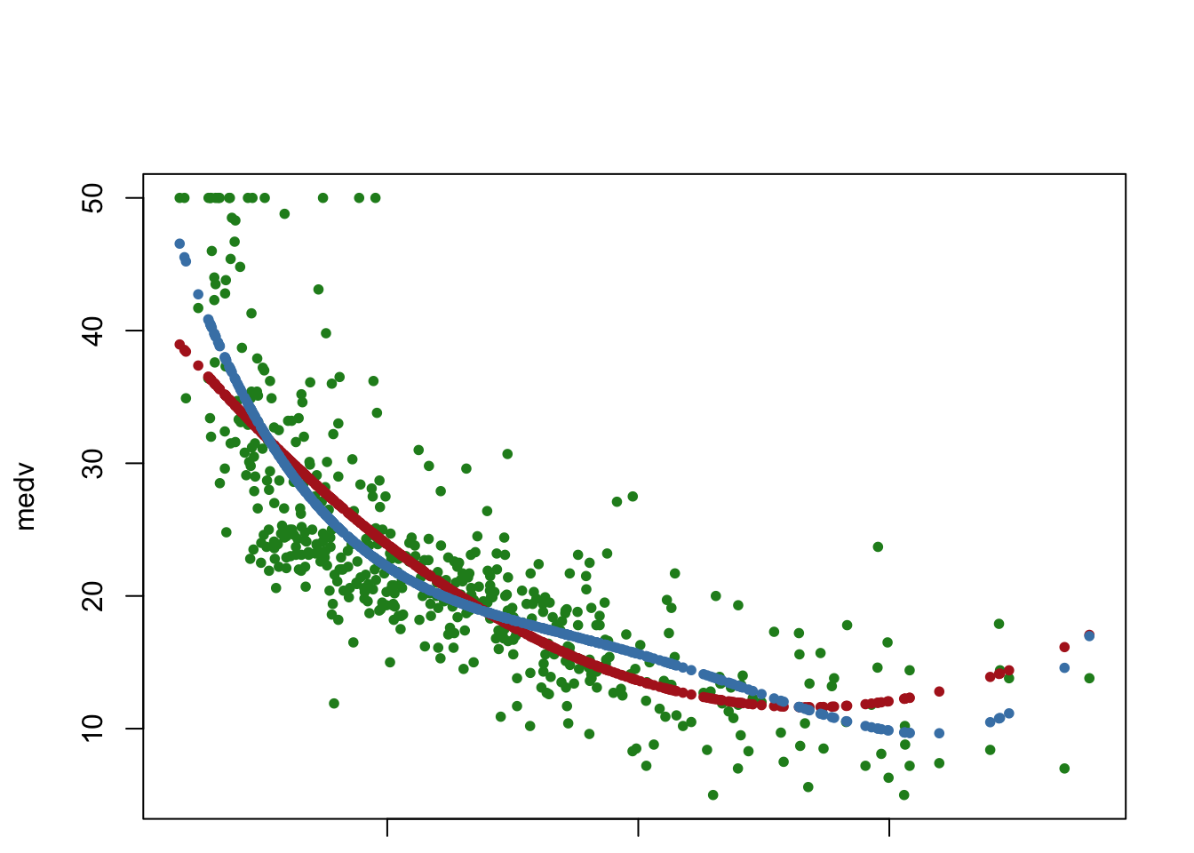
## I() identity function for squared term to interpret as-is## Combine two command lines with semicolonfit6=lm(medv~lstat +I(lstat^2),Boston); summary(fit6)
Call:
lm(formula = medv ~ lstat + I(lstat^2), data = Boston)

Residuals:
     Min       1Q   Median       3Q      Max
-15.2834  -3.8313  -0.5295   2.3095  25.4148

Coefficients:
             Estimate Std. Error t value Pr(>|t|)
(Intercept) 42.862007   0.872084   49.15   <2e-16 ***
lstat       -2.332821   0.123803  -18.84   <2e-16 ***
I(lstat^2)   0.043547   0.003745   11.63   <2e-16 ***
---
Signif. codes:  0 '***' 0.001 '**' 0.01 '*' 0.05 '.' 0.1 ' ' 1

Residual standard error: 5.524 on 503 degrees of freedom
Multiple R-squared:  0.6407,    Adjusted R-squared:  0.6393
F-statistic: 448.5 on 2 and 503 DF,  p-value: < 2.2e-16
     Sales          CompPrice       Income        Advertising
 Min.   : 0.000   Min.   : 77   Min.   : 21.00   Min.   : 0.000
 1st Qu.: 5.390   1st Qu.:115   1st Qu.: 42.75   1st Qu.: 0.000
 Median : 7.490   Median :125   Median : 69.00   Median : 5.000
 Mean   : 7.496   Mean   :125   Mean   : 68.66   Mean   : 6.635
 3rd Qu.: 9.320   3rd Qu.:135   3rd Qu.: 91.00   3rd Qu.:12.000
 Max.   :16.270   Max.   :175   Max.   :120.00   Max.   :29.000
   Population        Price        ShelveLoc        Age          Education
 Min.   : 10.0   Min.   : 24.0   Bad   : 96   Min.   :25.00   Min.   :10.0
 1st Qu.:139.0   1st Qu.:100.0   Good  : 85   1st Qu.:39.75   1st Qu.:12.0
 Median :272.0   Median :117.0   Medium:219   Median :54.50   Median :14.0
 Mean   :264.8   Mean   :115.8                Mean   :53.32   Mean   :13.9
 3rd Qu.:398.5   3rd Qu.:131.0                3rd Qu.:66.00   3rd Qu.:16.0
 Max.   :509.0   Max.   :191.0                Max.   :80.00   Max.   :18.0
 Urban       US
 No :118   No :142
 Yes:282   Yes:258
fit1=lm(Sales~.+Income:Advertising+Age:Price,Carseats) # add two interaction termssummary(fit1)
attach(Carseats)contrasts(Carseats$ShelveLoc) # what is contrasts function?
       Good Medium
Bad       0      0
Good      1      0
Medium    0      1
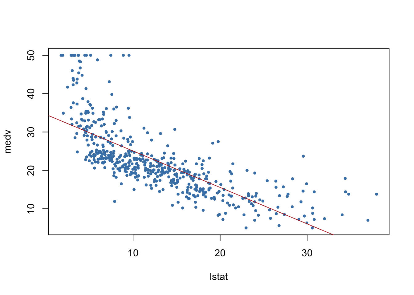
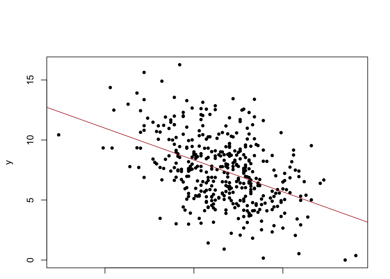
?contrasts### Writing an R function to combine the lm, plot and abline functions to ### create a one step regression fit plot functionregplot=function(x,y){ fit=lm(y~x)plot(x,y, pch=20)abline(fit,col="firebrick")}attach(Carseats)
The following objects are masked from Carseats (pos = 3):

    Advertising, Age, CompPrice, Education, Income, Population, Price,
    Sales, ShelveLoc, Urban, US
regplot(Price,Sales)
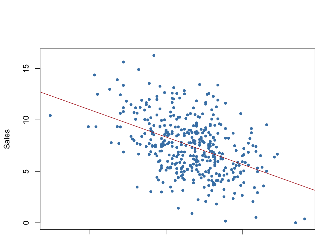
## Allow extra room for additional arguments/specificationsregplot=function(x,y,...){ fit=lm(y~x)plot(x,y,...)abline(fit,col="firebrick")}regplot(Price,Sales,xlab="Price",ylab="Sales",col="steelblue",pch=20)